Search Knowledge Base by Keyword
How to use Flat spreadsheet & formulas in it?
SUMMARY:
Electronic Lab Notebook (ELN), provides you with a rich text editor that allows you to use a page with many functions, like the photo, plate, chemistry editor, creating LabCollector links to reagents and supplies, copy-pasting from Word document directly, and many more. It also provides you with various spreadsheets for creating graphs. ELN provides you with 2 graphs: Flatspreadsheet (simple) and Zoho spreadsheet (more like excel).
Follow the steps below to start with the Flat spreadsheet:-
1. Shortcut guide
2. Formulas to use
3. Creating Graphs
![]()
1. Shortcut guide
- Flat spreadsheet allows to use Shortcuts guide that help you navigate through the flat spreadsheet.
- To open it go to HOME -> BOOK -> EXPERIMENT -> PAGE -> FLAT SPREADSHEET -> EDIT -> SHORTCUTS GUIDE.
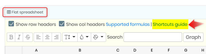
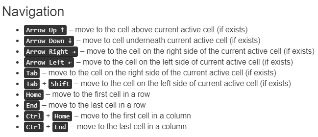
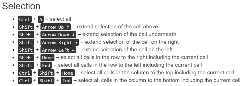
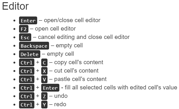
- When you click on “Shortcuts guide” you will see the below options.

![]()
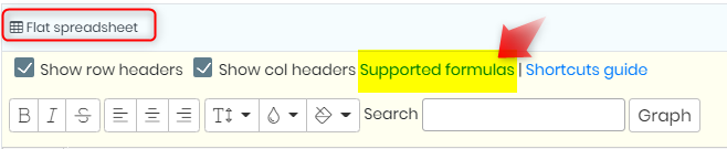
2. Formulas to use
- Flat spreadsheet allows to use Shortcuts guide that help you navigate through the flat spreadsheet.
- To open it go to HOME -> BOOK -> EXPERIMENT -> PAGE -> FLAT SPREADSHEET -> EDIT -> SUPPORTED FORMULAS.
- Formulas can be inserted in uppercase or lowercase (AVERAGE or average)
- Formulas work with either colon or semicolon between cell numbers.
- Syntax below, is the arrangement & explaination of the formula.
|
|
Formula |
Description |
|
1 |
ABS |
Absolute Value is a number is its value without the +/- sign. *You can only find the ABS for an individual cell at a time. |
|
2 |
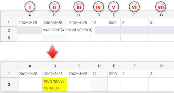
ACCRINT |
Calculates the accrued interest for a security with periodic interest payments. Syntax: ACCRINT(issue; first_interest; settlement; rate; par; frequency; basis) i. issue: the issue date of the security. ii. first_interest: the first interest date of the security. iii. settlement: the date at which the interest accrued up until then is to be calculated. iv. rate: the annual nominal rate of interest (coupon interest rate) v. par: the par value of the security. vi. frequency: the number of interest payments per year (1, 2 or 4). vii. basis: is chosen from a list of options and indicates how the year is to be calculated. Defaults to 0 if omitted. 0 – US method (NASD), 12 months of 30 days each 1 – Exact number of days in months, exact number of days in year 2 – Exact number of days in month, year has 360 days 3 – Exact number of days in month, year has 365 days 4 – European method, 12 months of 30 days each
|
|
3 |
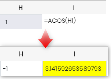
ACOS |
Returns the inverse cosine (the arccosine) of a number.
|
|
4 |
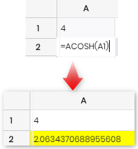
ACOSH |
Returns the inverse hyperbolic cosine of a number.
|
|
5 |
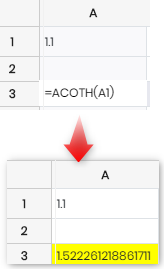
ACOTH |
Returns the inverse hyperbolic cotangent of the given number.
|
|
6 |
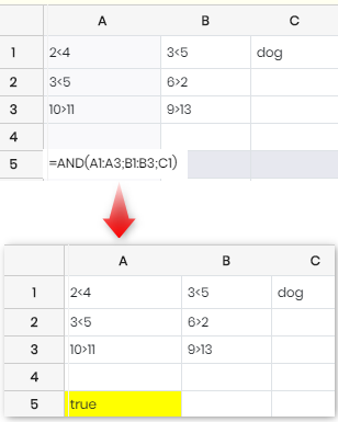
AND |
Returns TRUE if all the arguments are considered TRUE, and FALSE otherwise. AND tests every value (as an argument, or in each referenced cell), and returns TRUE if they are all TRUE. Any value which is a non-zero number or text is considered to be TRUE.
|
|
5 |
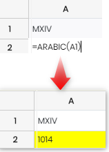
ARABIC |
Returns an Arabic number (eg 14), given a Roman number (eg XIV).
|
|
6 |
ASIN |
Returns the inverse tangent (the arctangent) of a number. E.g. to enter the formula in a cell put =ASIN(cell number) |
|
7 |
ASINH |
Returns the inverse sine (the arcsine) of a number. |
|
8 |
ATAN |
Returns the inverse tangent (the arctangent) of a number. E.g. to enter the formula in a cell put =ATAN(cell number) |
|
9 |
ATAN2 |
Returns the inverse tangent (the arctangent) for specified x and y coordinates. E.g. to enter the formula in a cell put =ATAN2(cell number) |
|
10 |
ATANH |
Returns the inverse hyperbolic tangent of a number. E.g. to enter the formula in a cell put =ATANH(cell number) |
|
11 |
AVEDEV |
Returns the average of the absolute deviations of values from their mean. E.g. to enter the formula in a cell put =AVEDEV(cell number:cell number:cell…) |
|
12 |
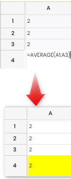
AVERAGE |
Returns the average of the arguments, ignoring text. E.g. to enter the formula in a cell put =AVERAGE(cell number:cell number:cell…)
|
|
13 |
AVERAGEA |
Returns the average of the arguments, including text (valued as 0). AVERAGEA(value1; value2; … value30) value1 to value30 are up to 30 values or ranges, which may include numbers, text and logical values. Text is evaluated as 0. Logical values are evaluated as 1 (TRUE) and 0 (FALSE). E.g. to enter the formula in a cell put =AVERAGE(cell number:cell number:cell number…) |
|
14 |
AVERAGEIF |
Returns the average (arithmetic mean) of all the cells in a range that meet a given criteria. E.g. to enter the formula in a cell put =AVERAGEIF(cell number:cell number:cell…) |
|
15 |
BASE |
Returns a text representation of a number, in a specified base radix. BASE(number; radix; minlength) converts number (a positive integer) to text, with the base radix (an integer between 2 and 36), using characters 0-9 and A-Z. minlength (optional) specifies the minimum number of characters returned; zeroes are added on the left if necessary. E.g. to enter the formula in a cell put =BASE(cell number:cell number:cell…) |
|
16 |
BESSELI |
Calculates the modified Bessel function of the first kind. BESSELI(x; n) returns the modified Bessel function of the first kind, of order n, evaluated at x. The modified Bessel function of the first kind In(x) = i-nJn(ix), where Jn is the * Bessel function of the first kind. E.g. to enter the formula in a cell put =BESSELI(cell number;cell number) |
|
17 |
BESSELJ |
Calculates the Bessel function of the first kind. BESSELJ(x; n) returns the Bessel function of the first kind, of order n, evaluated at x. The Bessel functions of the first kind Jn(x) are solutions to the Bessel differential equation. E.g. to enter the formula in a cell put =BESSELJ(cell number;cell number) |
|
18 |
BESSELK |
Calculates the modified Bessel function of the second kind. BESSELK(x; n) returns the modifed Bessel function of the second kind, of order n, evaluated at x. The modified Bessel functions of the second kind (also known as Basset functions) are often denoted Kn(x). E.g. to enter the formula in a cell put =BESSELJ(cell number;cell number) |
|
19 |
BESSELY |
Calculates the Bessel function of the second kind (the Neumann or Weber function). BESSELY(x; n) returns the Bessel function of the second kind, of order n, evaluated at x. The Bessel functions of the second kind Yn(x) (also known as Neumann Nn(x) or Weber functions) are solutions to the Bessel differential equation which are singular at the origin. E.g. to enter the formula in a cell put =BESSELY(cell number;cell number) |
|
20 |
BETADIST |
Calculates the cumulative distribution function or the probability density function of a beta distribution. You can read more about it from here. |
|
21 |
BETAINV |
Calculates the inverse of the BETADIST function. E.g. to enter the formula in a cell put =BETAINV(cell number;cell number) |
|
22 |
BIN2DEC |
Converts a binary number to decimal. E.g. to enter the formula in a cell put =BIN2DEC(cell number) |
|
23 |
BIN2HEX |
Converts a binary number to hexadecimal. E.g. to enter the formula in a cell put =BIN2HEX(cell number) |
|
24 |
BIN2OCT |
Converts a binary number to octal. E.g. to enter the formula in a cell put =BIN2OCT(cell number) |
|
25 |
BINOMDIST |
Calculates probabilities for a binomial distribution. BINOMDIST(k; n; p; mode) E.g. to enter the formula in a cell put =BINOMDIST(cell number; Cell number; cell number) |
|
26 |
BINOMDISTRANGE |
Calculated Binomial distribution range. E.g. =BINOM.DIST.RANGE(60,0.75,48) Returns the binomial distribution based on the probability of 48 successes in 60 trials and a 75% probability of success (0.084, or 8.4%). E.g. to enter the formula in a cell put =BINOMDISTRANGE(cell number:cell number:cell number) |
|
27 |
BINOMINV |
NOM.INV(trials,probability_s,alpha) The BINOM.INV function syntax has the following arguments: – Trials : Required. The number of Bernoulli trials. – Probability_s : Required. The probability of a success on each trial. – Alpha : Required. The criterion value. E.g. to enter the formula in a cell put =BINOMDINV(cell number:cell number:cell number) |
|
28 |
BITAND |
BITAND returns the bitwise and of the binary representations of its arguments. where a cell number is a non-negative integer. E.g. to enter the formula in a cell put =BITAND(cell number:cell number) |
|
29 |
BITLSHIFT |
returns the binary representations of a shifted n positions to the left. where one cell number is a non-negative integer & another cell number is an integer E.g. to enter the formula in a cell put =BITLSHIFT(cell number:cell number) |
|
30 |
BITOR |
returns the bitwise or of the binary representations of its arguments. E.g. to enter the formula in a cell put =BITOR(cell number;cell number) where the cell number is a non-negative integer |
|
31 |
BITRSHIFT |
returns the binary representations of a shifted n positions to the right. NOTE: If n is negative, BITRSHIFT shifts the bits to the left by ABS(n) positions. E.g. to enter the formula in a cell put =BITRSHIFT(cell number;cell number) where one cell number is a non-negative integer & another cell number is an integer |
|
32 |
BITXOR |
returns the bitwise exclusive or of the binary representations of its arguments. E.g. to enter the formula in a cell put =BITXOR(cell number;cell number) where the cell number is a non-negative integer |
|
33 |
CEILING |
Returns a number rounded up to a multiple of another number. Syntax: CEILING(number; mult; mode) – number is the number that is to be rounded up to a multiple of mult. – If mode is zero or omitted, CEILING rounds up to the multiple above (greater than or equal to) number. If mode is non-zero, CEILING rounds up away from zero. This is only relevant with negative numbers. Use mode=1 for compability if you have negative numbers and wish to export to MS Excel. In MS Excel this function only takes two arguments. to enter the formula put =CEILING(cell number;cell number;cell number) |
|
34 |
CEILINGMATH |
Rounds a number up to the nearest integer or to the nearest multiple of significance. Syntax: CEILING.MATH(number, [significance], [mode]) The CEILING.MATH function syntax has the following arguments. – Number *Required. Number must be less than 9.99E+307 and greater than -2.229E-308. – Significance *Optional. The multiple to which Number is to be rounded. – Mode *Optional. For negative numbers, controls whether Number is rounded toward or away from zero. to enter the formula put =CEILINGMATH(cell number:cell number:cell number) |
|
35 |
CEILINGPRECISE |
Rounds a number up to a given multiple. Unlike the CEILING function, CEILING.MATH defaults to a multiple of 1, and always rounds negative numbers toward zero. to enter the formula put =CEILING(cell number;cell number;cell number) where one cell number the one to be rounded and other is to put multiple to use when rounding. Default is 1. The second number is optional. |
|
36 |
CHAR |
Returns a single text character, given a character code. Syntax: CHAR(number) number is the character code, in the range 1-255. CHAR uses your system’s character mapping (for example iso-8859-1, iso-8859-2, Windows-1252, Windows-1250) to determine which character to return. Codes greater than 127 may not be portable. =CHAR(cell number) |
|
37 |
CHISQDIST |
Calculates values for a χ2-distribution. For more information please see this link. |
|
38 |
CHISQINV |
Calculates the inverse of the CHISQDIST function. Syntax: to enter the formula =CHISQINV(p; k) k is the degrees of freedom for the χ2-distribution. Constraint: k must be a positive integer p is the given probability Constraint: 0 ≤ p < 1 |
|
39 |
CODE |
returns the numeric code for the first character in a text string. Syntax: CODE(text) returns the numeric code for the first character of the text string text, in the range 0-255. Codes greater than 127 may depend on your system’s character mapping (for example iso-8859-1, iso-8859-2, Windows-1252, Windows-1250), and hence may not be portable to enter the formula =CODE(cell number) |
|
40 |
COMBIN |
Returns the number of combinations of a subset of items. Syntax: COMBIN(n; k) n is the number of items in the set. k is the number of items to choose from the set. COMBIN returns the number of ways to choose these items. For example if there are 3 items A, B and C in a set, you can choose 2 items in 3 different ways, namely AB, AC and BC. COMBIN implements the formula: n!/(k!(n–k)!) to enter the formula =COMBIN(cell number, cell number) |
|
41 |
COMBINA |
Returns the number of combinations of a subset of items. Syntax: COMBINA(n; k) n is the number of items in the set. k is the number of items to choose from the set. COMBINA returns the number of unique ways to choose these items, where the order of choosing is irrelevant, and repetition of items is allowed. For example if there are 3 items A, B and C in a set, you can choose 2 items in 6 different ways, namely AA, AB, AC, BB, BC and CC; you can choose 3 items in 10 different ways, namely AAA, AAB, AAC, ABB, ABC, ACC, BBB, BBC, BCC, CCC. COMBINA implements the formula: (n+k-1)!/(k!(n-1)!) to enter the formula =COMBINA(cell number, cell number) |
|
42 |
COMPLEX |
Returns a complex number, given real and imaginary parts. Syntax: COMPLEX(realpart; imaginarypart; suffix) returns a complex number as text, in the form a+bi or a+bj. realpart and imaginarypart are numbers. suffix is optional text i or j (in lowercase) to indicate the imaginary part of the complex number; it defaults to i. to enter the formula =COMPLEX (cell number, cell number, cell number) |
|
43 |
CONCATENATE |
Combines several text strings into one string. Syntax: CONCATENATE(text1; text2; … text30) returns up to 30 text strings text1 – text30, joined together. text1 – text30 may also be single cell references. he ampersand operator & may also be used to concatenate text in a formula, without the function. Read more about it from here. |
|
44 |
CONFIDENCENORM |
Returns the confidence interval for a population mean, using a normal distribution. Syntax: CONFIDENCE.NORM(alpha,standard_dev,size) The CONFIDENCE.NORM function syntax has the following arguments: – Alpha *Required. The significance level used to compute the confidence level. The confidence level equals 100*(1 – alpha)%, or in other words, an alpha of 0.05 indicates a 95 percent confidence level. – Standard_dev *Required. The population standard deviation for the data range and is assumed to be known. – Size *Required. The sample size. Read more about it from here. |
|
45 |
CONFIDENCET |
Returns the confidence interval for a population mean, using a Student’s t distribution. Syntax: CONFIDENCE.T(alpha,standard_dev,size) The CONFIDENCE.T function syntax has the following arguments: – Alpha *Required. The significance level used to compute the confidence level. The confidence level equals 100*(1 – alpha)%, or in other words, an alpha of 0.05 indicates a 95 percent confidence level. – Standard_dev *Required. The population standard deviation for the data range and is assumed to be known. – Size *Required. The sample size. Read more about it from here. |
|
46 |
CONVERT |
Converts legacy European national currencies to and from Euros. Syntax: CONVERT(value; currency1; currency2) value is the amount of the currency to be converted. currency1 and currency2 are the currency units to convert from and to respectively. These must be text, the official abbreviation for the currency (for example, “EUR”), as shown in the table below. The rates (shown per Euro) were set by the European Commission. The legacy currencies were replaced by the Euro in 2002. CONVERT(100;”ATS”;”EUR”) converts 100 Austrian Schillings into Euros. Read more about it from here. |
|
47 |
CORREL |
Returns the Pearson correlation coefficient of two sets of data. Syntax: CORREL(x; y) where x and y are ranges or arrays containing the two sets of data. Any text or empty entries are ignored. CORREL calculates: where are the averages of x,y. |
|
48 |
COS |
Returns the cosine of the given angle (in radians). Example: COS(PI()/2) returns 0, the cosine of PI/2 radians COS(RADIANS(60)) returns 0.5, the cosine of 60 degrees |
|
49 |
COSH |
Returns the hyperbolic cosine of a number. Syntax: COSH(number) returns the hyperbolic cosine of number. Example: COSH(0) returns 1, the hyperbolic cosine of 0. |
|
50 |
COT |
Returns the cotangent of the given angle (in radians). Syntax: COT(angle) returns the (trigonometric) cotangent of angle, the angle in radians. To return the cotangent of an angle in degrees, use the RADIANS function. The cotangent of an angle is equivalent to 1 divided by the tangent of that angle. Example: COT(PI()/4) returns 1, the cotangent of PI/4 radians. COT(RADIANS(45)) returns 1, the cotangent of 45 degrees. |
|
51 |
COTH |
Returns the hyperbolic cotangent of a number. Syntax: COTH(number) returns the hyperbolic cotangent of number. Example: COTH(1) returns the hyperbolic cotangent of 1, approximately 1.3130. |
|
52 |
COUNT |
Counts the numbers in the list of arguments, ignoring text entries. Syntax: COUNT(value1; value2; … value30) value1 to value30 are up to 30 values or ranges representing the values to be counted. Examples: COUNT(2; 4; 6; “eight”) returns 3, because 2, 4 and 6 are numbers (“eight” is text). |
|
53 |
COUNTA |
Counts the non-empty values in the list of arguments. Syntax: COUNTA(value1; value2; … value30) value1 to value30 are up to 30 values or ranges representing the values to be counted. Example: COUNTA(B1:B3) where cells B1, B2, B3 contain 1.1, =NA(), apple returns 3, because none of the cells in B1:B3 are empty. |
|
54 |
COUNTBLANK |
Returns the number of empty cells. Syntax: COUNTBLANK(range) Returns the number of empty cells in the cell range range. A cell that contains blank text such as spaces, or even text with zero length such as returned by =””, is not considered empty, even though it may appear empty. Example: COUNTBLANK(A1:B2) returns 4 if cells A1, A2, B1 and B2 are all empty. |
|
55 |
COUNTIF |
Counts the number of cells in a range that meet a specified condition. Syntax: COUNTIF(test_range; condition) test_range is the range to be tested. Example: COUNTIF(C2:C8; “>=20”) returns the number of cells in C2:C8 whose contents are numerically greater than or equal to 20. Read more about it from here. |
|
56 |
COUNTIFS |
The COUNTIFS function applies criteria to cells across multiple ranges and counts the number of times all criteria are met. Syntax: COUNTIFS(criteria_range1, criteria1, [criteria_range2, criteria2]…) The COUNTIFS function syntax has the following arguments: criteria_range1 *Required. The first range in which to evaluate the associated criteria. criteria1 *Required. The criteria in the form of a number, expression, cell reference, or text that define which cells will be counted. For example, criteria can be expressed as 32, “>32”, B4, “apples”, or “32”. criteria_range2, criteria2, … *Optional. Additional ranges and their associated criteria. Up to 127 range/criteria pairs are allowed. |
|
58 |
COUNTUNIQUE |
Counts the number of unique values in a list of specified values and ranges. Syntax: COUNTUNIQUE(value1, [value2, …]) · value1 – The first value or range to consider for uniqueness. · value2, … – [ OPTIONAL ] – Additional values or ranges to consider for uniqueness. |
|
59 |
COVARIANCEP |
This article describes the formula syntax and usage of the COVARIANCE.P function in Microsoft Excel. Returns population covariance, the average of the products of deviations for each data point pair in two data sets. Use covariance to determine the relationship between two data sets. For example, you can examine whether greater income accompanies greater levels of education. Syntax: COVARIANCE.P(array1,array2) The COVARIANCE.P function syntax has the following arguments: Array1 Required. The first cell range of integers. Array2 Required. The second cell range of integers. Read about it from here. |
|
60 |
COVARIANCES |
Returns the sample covariance, the average of the products of deviations for each data point pair in two data sets. Syntax: COVARIANCE.S(array1,array2) The COVARIANCE.S function syntax has the following arguments: Array1 Required. The first cell range of integers. Array2 Required. The second cell range of integers. Read about it from here. |
|
61 |
CSC |
Returns the cosecant of a number Syntax: SC(number) returns the cosecant of number. Example: CSC(0): returns 1, the cosecant of 0. |
|
62 |
CSCH |
Returns the hyperbolic cosecant of a number. Syntax: CSCH(number) returns the hyperbolic cosecant of number. Example: CSCH(0): returns 1, the hyperbolic cosecant of 0. |
|
63 |
CUMIPMT |
Returns the total interest paid on a loan in specified periodic payments. Syntax: CUMIPMT(rate; numperiods; presentvalue; start; end; type) rate: the interest rate per period. numperiods: the total number of payment periods in the term. presentvalue: the initial sum borrowed. start: the first period to include. Periods are numbered beginning with 1. end: the last period to include. type: when payments are made: 0 – at the end of each period. 1 – at the start of each period (including a payment at the start of the term). Read about it from here. |
|
64 |
CUMPRINC |
Returns the total capital repaid on a loan in specified periodic payments. Syntax: CUMPRINC(rate; numperiods; presentvalue; start; end; type) – rate: the interest rate per period. – numperiods: the total number of payment periods in the term. – presentvalue: the initial sum borrowed. – start: the first period to include. Periods are numbered beginning with 1. – end: the last period to include. – type: when payments are made: 0 – at the end of each period. 1 – at the start of each period (including a payment at the start of the term). Read about it from here. |
|
65 |
DATE |
DATE(year; month; day) returns the date, expressed as a date-time serial number. year is an integer between 1583 and 9956 or between 0 and 99; month and day are integers. If month and day are not within range for a valid date, the date will ‘roll over’, as shown below. Example: DATE(2007; 11; 9) returns the date 9th November 2007 (as a date-time serial number). DATE(2007; 12; 32) returns 1st January 2008 – the date rolls over, as 32nd December 2007 is not valid. |
|
66 |
DATEVALUE |
returns the date-time serial number, from a date given as text. Syntax: DATEVALUE(datetext) datetext is a date, expressed as text. DATEVALUE returns the date-time serial number, which may be formatted to read as a date. Example: DATEVALUE(“2007-11-23”) returns 39409, the date-time serial number for 23Nov2007 (assuming the default date-time starting date) |
|
67 |
DAY |
Returns the day of a given date. Syntax: DAY(date) returns the day of date as a number (1-31). date may be text or a date-time serial number. DAY(“2008-06-04”) returns 4. |
|
68 |
DAYS |
Returns the number of days between two dates Syntax: DAYS(enddate; startdate) startdate and enddate may be dates as numbers or text (which is converted to number form). DAYS returns enddate – startdate. The result may be negative. Example: DAYS(“2008-03-03”; “2008-03-01”) returns 2, the number of days between 1March08 and 3March08. DAYS(A1; A2) where cell A1 contains the date 2008-06-09 and A2 contains 2008-06-02 returns 7. |
|
69 |
DAYS360 |
Returns the number of days between two dates, using the 360 day year. Syntax: DAYS360(enddate; startdate; method) startdate and enddate are the starting and ending dates (text or date-time serial numbers). If startdate is earlier than enddate, the result will be negative. method is an optional parameter; if 0 or omitted, the US National Association of Securities Dealers (NASD) method of calculation is used; if 1 (or <>0) the European method of calcuation is used. The calculation assumes that all months have 30 days, so a year (12 months) has 360 days. See Financial date systems for more details. Example: DAYS360(“2008-02-29”; “2008-08-31”) returns 180, that is, 6 months of 30 days. |
|
70 |
DB |
Returns the depreciation of an asset for a given year using the fixed rate declining-balance method. Syntax: DB(originalcost; salvagevalue; lifetime; year; months1styear) originalcost: the initial cost of the asset. salvagevalue: is the value at the end of the depreciation (sometimes called the salvage value of the asset). lifetime: the number of years over which the asset is being depreciated. year: the year number for which the depreciation is calculated. months1styear: the number of months in the first year (defaults to 12 if omitted). Read about it from here. |
|
71 |
DDB |
Returns the depreciation of an asset for a given year using the double (or other factor) declining-balance method. Syntax: DDB(originalcost; salvagevalue; lifetime; year; factor) originalcost: the initial cost of the asset. salvagevalue: is the value at the end of the depreciation (sometimes called the salvage value of the asset). lifetime: the number of years over which the asset is being depreciated. year: the year number for which the depreciation is calculated. factor: the factor to set the depreciation rate (2 if omitted). Read about it from here. |
|
72 |
DEC2BIN |
Converts a decimal number to binary. Syntax: DEC2BIN(number; numdigits) returns a binary number as text, given the decimal number, which must be between -512 and 511 inclusive, and may be text or a number. The output is a binary number with up to ten bits in two’s complement representation; positive numbers are 0 to 111111111 (nine bits representing 0 to 511 decimal) and negative numbers 1111111111 to 1000000000 (ten bits representing -1 to -512 decimal). numdigits is an optional number specifying the number of digits to return. Example: DEC2BIN(9) returns 1001 as text. DEC2BIN(“9”) returns 1001 as text. DEC2BIN will accept a decimal number given as text. |
|
73 |
DEC2HEX |
Converts a decimal number to hexadecimal. Syntax: DEC2HEX(number; numdigits) returns a hexadecimal number as text, given the decimal number, which must be between -239 and 239-1 inclusive, and may be text or a number. The output is a hexadecimal number with up to ten digits in two’s complement representation. numdigits is an optional number specifying the number of digits to return. Example: DEC2HEX(30) returns 1E as text. DEC2HEX(“30”) returns 1E as text. DEC2HEX will accept a decimal number given as text. |
|
74 |
DEC2OCT |
Converts a decimal number to octal. Syntax: DEC2OCT(number; numdigits) returns an octal number as text, given the decimal number, which must be between -229 and 229-1 inclusive, and may be text or a number. The result is an octal number with up to ten digits in two’s complement representation. numdigits is an optional number specifying the number of digits to return. Example: DEC2OCT(19) returns 23 as text. DEC2OCT(“19”) returns 23 as text. DEC2OCT will accept a decimal number given as text. |
|
75 |
DECIMAL |
Returns a decimal number, given a text representation and its base radix. Syntax: DECIMAL(text; radix) text is text representing a number with the base radix radix (an integer between 2 and 36). Any leading spaces and tabs are ignored. Letters, if any, may be upper or lower case. If radix is 16 (hexadecimal system), any leading 0x, 0X, x or X is ignored, as is any trailing h or H. If radix is 2 (binary system), any trailing b or B is ignored. Example: DECIMAL(“00FF”; 16) returns 255 as a number (hexadecimal system). |
|
76 |
DEGREES |
Converts radians into degrees. Syntax: DEGREES(radians) radians is the angle in radians to be converted to degrees. Example: DEGREES(PI()) returns 180 degrees |
|
77 |
DELTA |
Returns 1 if two numbers are equal, and 0 otherwise. Syntax: DELTA(number1; number2) number1 and number2 are numbers. If number2 is omitted it is assumed to be 0. This function is an implementation of the (mathematical) Kronecker delta function. number1=number2 returns TRUE or FALSE instead of 1 or 0, but is otherwise identical for number arguments. Example: DELTA(4; 5) returns 0. DELTA(4; A1) where cell A1 contains 4, returns 1. |
|
78 |
DEVSQ |
Returns the sum of squares of deviations from the mean. Syntax: DEVSQ(number1; number2; … number30) number1 to number30 are up to 30 numbers or ranges containing numbers. DEVSQ calculates the mean of all the numbers, then sums the squared deviation of each number from that mean. With N values, the calculation formula is: Example: DEVSQ(1; 3; 5) returns 8, calculated as (-2)2 + 0 + (2)2. |
|
79 |
DOLLAR |
Returns text representing a number in your local currency format. Syntax: DOLLAR(number; decimals) returns text representing number as currency. decimals (optional, assumed to be 2 if omitted) sets the number of decimal places. Tools – Options – Language Settings – Languages – ‘Default Currency’ sets the currency to be used (normally be the currency of your locale). Example: DOLLAR(255) returns $255.00, if your currency is US dollars. DOLLAR(367.456; 2) returns $367.46, if your currency is US dollars. |
|
80 |
DOLLARDE |
Converts a fractional number representation of a number into a decimal number. Syntax: DOLLARDE(fractionalrep; denominator) fractionalrep: the fractional representation. Sometimes a security price, for example, might be expressed as 2.03, meaning $2 and 3/16 of a dollar. denominator: the denominator – for example, 16 in the example above. DOLLARDE converts the fractional representation to decimal. Despite its name, it returns a number, not a currency. Its inverse is DOLLARFR. Example: DOLLARDE(2.03; 16) returns 2.1875 as a number. 2 + 3/16 equals 2.1875. |
|
81 |
DOLLARFR |
Converts a decimal number into a fractional representation of that number. Syntax: DOLLARFR(decimal; denominator) decimal: the decimal number. denominator: the denominator for the fractional representation. Sometimes a security price, for example, might be expressed as 2.03, a fractional representation meaning $2 and 3/16 of a dollar. As a decimal this is 2.1875. DOLLARFR converts the decimal representation to a fractional representation. Despite its name, it returns a number, not a currency. Its inverse is DOLLARDE. Example: DOLLARFR(2.1875; 16) returns 2.03 as a number. 2 + 3/16 equals 2.1875. |
|
83 |
EDATE |
Returns a date a number of months away. Syntax: EDATE(startdate; months) months is a number of months that are added to the startdate. The day of the month remains unchanged, unless it is more than the number of days in the new month (when it becomes the last day of that month). months may be negative. Example: EDATE(“2008-10-15”; 2) returns 15Dec08. EDATE(“2008-05-31”; -1) returns 30Apr08. There are only 30 days in April. |
|
84 |
EFFECT |
Calculates the annual effective interest rate given the nominal rate and number of compounding periods per year. Syntax: EFFECT(nominal_rate, periods_per_year) · nominal_rate – The nominal interest rate per year. · periods_per_year – The number of compounding periods per year. Read about it from here. |
|
85 |
EOMONTH |
Returns the date of the last day of a month. Syntax: EOMONTH(startdate; addmonths) addmonths is a number of months to be added to the startdate (given as text or a date-time serial number), to give a new date. For this new date, EOMONTH returns the date of the last day of the month, as a date-time serial number. addmonths may be positive (in the future), zero or negative (in the past). Example: EOMONTH(“2008-02-14”; 0) returns 39507, which may be formatted as 29Feb08. 2008 is a leap year. |
|
86 |
ERF |
Calculates the error function (Gauss error function). Syntax: ERF(number1; number2) if number2 is omitted, returns the error function calculated between 0 and number1, otherwise returns the error function calculated between number1 and number2. The error function, also known as the Gauss error function, is defined for ERF(x) as: ERF(x1; x2) is ERF(x2) – ERF(x1). Example: ERF(0.5) returns 0.520499877813. ERF(0.2; 0.5) returns 0.297797288603. |
|
87 |
ERFC |
Calculates the complementary error function (complementary Gauss error function). Syntax: ERFC(number) returns the error function calculated between number and infinity, that is, the complementary error function for number. ERFC(x) = 1 – ERF(x). Example: ERFC(0.5) returns 0.479500122187 |
|
88 |
EVEN |
Rounds a number up, away from zero, to the next even integer. Syntax: EVEN(number) returns number rounded to the next even integer up, away from zero. Example: EVEN(2.3) returns 4. |
|
89 |
EXACT |
Returns TRUE if two text strings are identical Syntax: EXACT(text1; text2) returns TRUE if the text strings text1 and text2 are exactly the same (including case). Example: EXACT(“red car”; “red car”) returns TRUE. EXACT(“red car”; “Red Car”) returns FALSE. |
|
90 |
EXPONDIST |
Calculates values for an exponential distribution. Syntax: EXPONDIST(x; λ; mode) The exponential distribution is a continuous probability distribution, with parameter λ (rate). λ must be greater than zero. If mode is 0, EXPONDIST calculates the probability density function of the exponential distribution: If mode is 1, EXPONDIST calculates the cumulative distribution function of the exponential distribution: Example: EXPONDIST(0; 1; 0) returns 1. EXPONDIST(0; 1; 1) returns 0. |
|
91 |
FALSE |
Returns the logical value FALSE. Syntax: FALSE() The FALSE() function has no arguments, and always returns the logical value FALSE. Example: FALSE() returns FALSE NOT(FALSE()) returns TRUE |
|
92 |
FDIST |
Calculates values for an F-distribution. Syntax: FDIST(x; r1; r2) r1 and r2, which are positive integers, are the degrees of freedom parameters for the F-distribution. x must be greater than or equal to 0. FDIST returns the area of the right tail of the probability density function for the F-distribution, calculating: Example: FDIST(1; 4; 5) returns approximately 0.485657. |
|
93 |
FINV |
Calculates the inverse of the FDIST function. Syntax: FINV(p; r1; r2) returns the value x, such that FDIST(x; r1; r2) is p. Parameters r1 and r2 (degrees of freedom) are positive integers. p must be greater than 0 and less than or equal to 1. Example: FINV(0.485657; 4; 5) returns approximately 1. |
|
94 |
FISHER |
Calculates values for the Fisher transformation. Syntax: FISHER(r) returns the value of the Fisher transformation at r, (-1 < r < 1). This function calculates: Example: FISHER(0) returns 0. |
|
95 |
FISHERINV |
Calculates the inverse of the FISHER transformation. Syntax: FISHERINV(z) returns the value r, such that FISHER(r) is z. This function calculates: Example: FISHERINV(0) returns 0. |
|
96 |
IF |
The IF function is one of the most popular functions in Excel, and it allows you to make logical comparisons between a value and what you expect. For more info please check here |
|
97 |
INT |
Rounds a number down to the nearest integer. Syntax: INT(number) returns number rounded down to the nearest integer. Negative numbers round down to the integer below: -1.3 rounds to -2. Example: INT(5.7) returns 5 INT(-1.3) returns -2. |
|
98 |
ISEVEN |
Returns TRUE if the value is an even number, or FALSE if the value is odd. Syntax: ISEVEN(value) value is the value to be checked. If value is not an integer any digits after the decimal point are ignored. The sign of value is also ignored. Example: ISEVEN(48) returns TRUE. ISEVEN(33) returns FALSE. |
|
99 |
ISODD |
Returns TRUE if the value is an odd number, or FALSE if the value is even. Syntax: ISODD(value) value is the value to be checked. If value is not an integer any digits after the decimal point are ignored. The sign of value is also ignored. Example: ISODD(33) returns TRUE. ISODD(48) returns FALSE. |
|
100 |
LN |
Returns the natural logarithm of a number. Syntax: LN(number) returns the natural logarithm (the logarithm to base e) of number, that is the power of e necessary to equal number. The mathematical constant e is approximately 2.71828182845904. Example: LN(3) returns the natural logarithm of 3 (approximately 1.0986). |
|
101 |
LOG |
Returns the logarithm of a number to the specified base. Syntax: LOG(number; base) returns the logarithm to base base of number. Example: LOG(10; 3) returns the logarithm to base 3 of 10 (approximately 2.0959). |
|
102 |
LOG10 |
Returns the base-10 logarithm of a number. Syntax: LOG10(number) returns the logarithm to base 10 of number. Example: LOG10(5) returns the base-10 logarithm of 5 (approximately 0.69897). |
|
103 |
MAX |
Returns the maximum of a list of arguments, ignoring text entries. Syntax: MAX(number1; number2; … number30) number1 to number30 are up to 30 numbers or ranges containing numbers. Example: MAX(2; 6; 4) returns 6, the largest value in the list. |
|
104 |
MAXA |
Returns the maximum of a list of arguments, including text and logical entries. Syntax: MAXA(value1; value2; … value30) value1 to value30 are up to 30 values or ranges, which may include numbers, text and logical values. Text is evaluated as 0. Logical values are evaluated as 1 (TRUE) and 0 (FALSE). Example: MAXA(2; 6; 4) returns 6, the largest value in the list. |
|
105 |
MEDIAN |
Returns the median of a set of numbers. Syntax: MEDIAN(number1; number2; … number30) number1 to number30 are up to 30 numbers or ranges containing numbers. MEDIAN returns the median (middle value) of the numbers. If the count of numbers is odd, this is the exact middle value. If the count of numbers is even, the average of the two middle values is returned. Example: MEDIAN(1; 5; 9; 20; 21) returns 9, the number exactly in the middle. |
|
106 |
MIN |
Returns the minimum of a list of arguments, ignoring text entries. Syntax: MIN(number1; number2; … number30) number1 to number30 are up to 30 numbers or ranges containing numbers. Example: MIN(2; 6; 4) returns 2, the smallest value in the list. MIN(B1:B3) where cells B1, B2, B3 contain 1.1, 2.2, and apple returns 1.1. |
|
107 |
MINA |
Returns the minimum of a list of arguments, including text and logical entries. Syntax: MINA(value1; value2; … value30) value1 to value30 are up to 30 values or ranges, which may include numbers, text and logical values. Text is evaluated as 0. Logical values are evaluated as 1 (TRUE) and 0 (FALSE). Example: MINA(2; 6; 4) returns 2, the smallest value in the list. MINA(B1:B3) where cells B1, B2, B3 contain 3, 4, and apple returns 0, the value of the text. |
|
108 |
MOD |
Returns the remainder when one integer is divided by another. Syntax: MOD(number; divisor) For integer arguments this function returns number modulo divisor, that is the remainder when number is divided by divisor. This function is implemented as number – divisor * INT( number/divisor) , and this formula gives the result if the arguments are not integer. Example: MOD(22; 3) returns 1, the remainder when 22 is divided by 3. |
|
109 |
NOT |
Reverses the logical value. Returns TRUE if the argument is FALSE, and FALSE if the argument is TRUE. Syntax: NOT(logical_value) where logical_value is the logical value to be reversed. Example: NOT( TRUE() ) returns FALSE |
|
110 |
ODD |
Rounds a number up, away from zero, to the next odd integer. Syntax: ODD(number) returns number rounded to the next odd integer up, away from zero. Example: ODD(1.2) returns 3. |
|
111 |
OR |
Returns TRUE if any of the arguments are considered TRUE, and FALSE otherwise. Syntax: OR(argument1; argument2 …argument30) argument1 to argument30 are up to 30 arguments, each of which may be a logical result or value, or a reference to a cell or range. OR tests every value (as an argument, or in a each referenced cell), and returns TRUE if any of them are TRUE. Any non-zero number is considered to be TRUE. Any text cells in ranges are ignored. Example: OR(TRUE; FALSE) returns TRUE. |
|
112 |
PI |
Returns 3.14159265358979, the value of the mathematical constant PI to 14 decimal places. Syntax: PI() Example: PI() returns 3.14159265358979 |
|
113 |
POWER |
Returns a number raised to a power. Syntax: POWER(number; power) returns numberpower, that is number raised to the power of power. The same result may be achieved by using the exponentiation operator ^: number^power Example: POWER(4; 3) returns 64, which is 4 to the power of 3. |
|
114 |
ROUND |
Rounds a number to a certain precision. Syntax: ROUND(number; places) returns number rounded to places decimal places. If places is omitted or zero, the function rounds to the nearest integer. If places is negative, the function rounds to the nearest 10, 100, 1000, etc. This function rounds to the nearest number. See ROUNDDOWN and ROUNDUP for alternatives. Example: ROUND(2.348; 2) returns 2.35 ROUND(2.348; 0) returns 2 |
|
115 |
ROUNDDOWN |
Rounds a number down, toward zero, to a certain precision. Syntax: ROUNDDOWN(number; places) returns number rounded down (towards zero) to places decimal places. If places is omitted or zero, the function rounds down to an integer. If places is negative, the function rounds down to the next 10, 100, 1000, etc. This function rounds towards zero. See ROUNDUP and ROUND for alternatives. Example: ROUNDDOWN(1.234; 2) returns 1.23 |
|
116 |
ROUNDUP |
Rounds a number up, away from zero, to a certain precision. Syntax: ROUNDUP(number; places) returns number rounded up (away from zero) to places decimal places. If places is omitted or zero, the function rounds up to an integer. If places is negative, the function rounds up to the next 10, 100, 1000, etc. This function rounds away from zero. See ROUNDDOWN and ROUND for alternatives. Example: ROUNDUP(1.1111; 2) returns 1.12 ROUNDUP(1.2345; 1) returns 1.3 |
|
117 |
SIN |
Returns the sine of the given angle (in radians). Syntax: SIN(angle) returns the (trigonometric) sine of angle, the angle in radians. To return the sine of an angle in degrees, use the RADIANS function. Example: SIN(PI()/2) returns 1, the sine of PI/2 radians SIN(RADIANS(30)) returns 0.5, the sine of 30 degrees |
|
118 |
SINH |
Returns the hyperbolic sine of a number. Syntax: SINH(number) returns the hyperbolic sine of number. Example: SINH(0) returns 0, the hyperbolic sine of 0. |
|
119 |
SPLIT |
Returns a zero-based, one-dimensional array containing a specified number of substrings. For more information read here. |
|
120 |
SQRT |
Returns the positive square root of a number. Syntax: SQRT(number) Returns the positive square root of number. number must be positive. Example: SQRT(16) returns 4. SQRT(-16) returns an invalid argument error. |
|
121 |
SQRTPI |
Returns the square root of (PI times a number). Syntax: SQRTPI(number) Returns the positive square root of ( PI multiplied by number ). This is equivalent to SQRT(PI()*number). Example: SQRTPI(2) returns the square root of (2PI), approximately 2.506628. |
|
122 |
SUM |
Sums the contents of cells. Syntax: SUM(number1; number2; … number30) number1 to number30 are up to 30 numbers or ranges/arrays of numbers whose sum is to be calculated. SUM ignores any text or empty cell within a range or array. SUM can also be used to sum or count cells where a specified condition is true – see Conditional Counting and Summation. Example: SUM(2; 3; 4) returns 9, because 2+3+4 = 9. |
|
123 |
SUMIF |
Conditionally sums the contents of cells in a range. Syntax: SUMIF(test_range; condition; sum_range) This function identifies those cells in the range test_range that meet the condition, and sums the corresponding cells in the range sum_range. If sum_range is omitted the cells in test_range are summed. For more info read here. |
|
124 |
SUMIFS |
adds all of its arguments that meet multiple criteria. For example, you would use SUMIFS to sum the number of retailers in the country who (1) reside in a single zip code and (2) whose profits exceed a specific dollar value. For more information read here. |
|
125 |
SUMPRODUCT |
Returns the sum of the products of corresponding array elements. Syntax: SUMPRODUCT(array1; array2; … array30) array1 to array30 are up to 30 arrays or ranges of the same size whose corresponding elements are to be multiplied. SUMPRODUCT returns for the i elements in the arrays. You can use SUMPRODUCT to calculate the scalar product of two vectors. Example: SUMPRODUCT(A1:B2; F1:G2) returns A1*F1 + B1*G1 + A2*F2 + B2*G2. Read more about it here. |
|
126 |
SUMSQ |
Returns the sum of the squares of the arguments. Syntax: SUMSQ(number1; number2; …. number30) number1 to number30 are up to 30 numbers or ranges of numbers which are squared and then summed. Example: SUMSQ(2; 3; 4) returns 29, which is 2*2 + 3*3 + 4*4. |
|
127 |
SUMX2MY2 |
Returns the sum of the differences between corresponding squared elements of two matrices. Syntax: SUMX2MY2(x; y) x and y are arrays or ranges of the same size. SUMX2MY2 calculates for the i elements in the arrays. Advanced topic: SUMX2MY2 evaluates its parameters x and y as array formulas but does not need to be entered as an array formula. In other words it can be entered with the Enter key, rather than Cntrl-Shift-Enter. See the example below. Example: SUMX2MY2(A1:A2; {2|1}) where cells A1 and A2 contain 4 and 3 respectively, returns (42-22) + (32-12) = 20. Read more about it here. |
|
128 |
SUMX2PY2 |
Returns the sum of the squares of all elements of two matrices. Syntax: SUMX2PY2(x; y) x and y are arrays or ranges of the same size. SUMX2PY2 calculates for the i elements in the arrays or ranges. Advanced topic: SUMX2PY2 evaluates its parameters x and y as array formulas but does not need to be entered as an array formula. In other words it can be entered with the Enter key, rather than Cntrl-Shift-Enter. See the example below. Example: SUMX2PY2(A1:A2; {2|1}) where cells A1 and A2 contain 4 and 3 respectively, returns (42+22) + (32+12) = 30. Read about it more here. |
|
129 |
SUMXMY2 |
Returns the sum of the squared differences between corresponding elements of two matrices. Syntax: SUMXMY2(x; y) x and y are arrays or ranges of the same size. SUMXMY2 calculates for the i elements in the arrays. |
|
130 |
TAN |
Returns the tangent of the given angle (in radians). Syntax: TAN(angle) returns the (trigonometric) tangent of angle, the angle in radians. To return the tangent of an angle in degrees, use the RADIANS function. Example: TAN(PI()/4) returns 1, the tangent of PI/4 radians. |
|
131 |
TANH |
Returns the hyperbolic tangent of a number. Syntax: TANH(number) returns the hyperbolic tangent of number. Example: TANH(0) returns 0, the hyperbolic tangent of 0. |
|
132 |
TRUE |
Returns the logical value TRUE. Syntax: TRUE() The TRUE() function has no arguments, and always returns the logical value TRUE. Example: TRUE() returns TRUE |
|
133 |
TRUNC |
Truncates a number by removing decimal places. Syntax: TRUNC(number; places) returns number with at most places decimal places. Excess decimal places are simply removed, irrespective of sign. TRUNC(number; 0) behaves as INT(number) for positive numbers, but effectively rounds towards zero for negative numbers. Example: TRUNC(1.239; 2) returns 1.23. The 9 is lost. |
|
134 |
XOR |
The XOR function returns a logical Exclusive Or of all arguments. Syntax: XOR(logical1, [logical2],…) The XOR function syntax has the following arguments. Logical1, logical2,… Logical 1 is required, subsequent logical values are optional. 1 to 254 conditions you want to test that can be either TRUE or FALSE, and can be logical values, arrays, or references. Please read this link for more information. |
![]()
3. Creating Graphs
- Please refer to the KB to see how to create the graph in flat spreadsheet.
![]()
Related topics:
- Please read our KB to see what is zoho spreadsheet and how to enable it.
- Please read our KB to know more about how to create graph in flat Spreadsheet.
- Read our manual on LabCollector.
- Check our KB on ELN template.
- Read about how ELN Workflow.
- Read more on how to create book, experiment & page
- Read our KB to know how to use rich text editor in ELN.
- Check our KB to read about what’s inside an experiment in ELN.
- Read what’s inside a book in ELN.
